A filtered NVDA options-chain corpus from OptionsDX — 753 trading days from 2019–2021, 432,529 contract records that passed OTM, maturity, quote and IV-quality screens (about 574 per day). Compiling an implied-volatility surface — 4 moneyness bands × 3 maturities, 12 cells in all — does not actually need the full chain: drop half, or even three quarters, and the surface still compiles. The only question is which contracts to drop. One clarification up front: the “surface” here is the grid of these 12 cell-mean IVs, not a continuously parameterised fit of the SVI type; what this article evaluates is the sampling reconstruction accuracy of cell means.

Bastola and Prushansky’s paper (arXiv:2610.33438) moves the problem into the survey-sampling frame: an options chain is a finite population, compiling a surface is estimating cell means, and a sampling design must first answer “what is the target?”. Their answer is crisp: for an equal-weighted surface, allocate stratified draws by each cell’s previous-day dispersion; for a liquidity-weighted surface, use liquidity PPS (probability proportional to size); get it wrong and the error multiplies.

I re-ran the whole protocol on a synthetic options chain with known ground truth: the core equal-weight claims replicated, the direction of the mismatch penalty replicated — but the paper’s prettiest sentence, “wins by construction”, did not replicate as stated. In my population, liquidity PPS still beats random sampling on its own matched target (ratios 0.50–0.81), yet loses at every retention rate to the plainest equal-cell stratification: what lost was the word “inevitable”, not PPS itself. This article covers three things: why alignment pays, why the wrong design doubles the error, and why “necessary by construction” only holds when target and budget live at the same level.

Boundaries first: every number in the paper comes from a single underlying, NVDA, all author-reported, across three different data spans (longitudinal 2018–2025, cross-sectional corpus 2019–2021, intraday 2022–2025); my re-test uses a synthetic population and examines mechanism and ordering, not NVDA magnitudes. I did not test the paper’s longitudinal training-equivalence or IV-forecasting parts; wherever they appear below, they are marked author-reported.

The paper’s protocol: name the target first, then sample

The paper’s cross-sectional study (§3) has four designs. Uniform random sampling (SRS) is the baseline. Liquidity PPS gives each contract a size (w=(\text{volume}+1)/(\text{relative spread}+10^{-4})); inclusion probability is proportional to (w), truncated at 1 for certainty units, and draws are taken with Madow systematic sampling (equally spaced points on the cumulative-probability scale).

The other two are stratified designs: split by the 4×3 grid first, then allocate using the previous trading day’s within-cell IV standard deviation (lagged one day, against look-ahead) — Neyman allocation (n_h \propto N_h S_{h,t-1}) for the population-weighted target, equal-cell allocation (n_h \propto S_{h,t-1}) for the 12-cell equal-weight target (allocation by lagged within-cell dispersion, not the same count per cell). The estimator switches with the target: Hájek for equal weight, a Horvitz–Thompson ratio estimator for liquidity weight. Both are weight-normalised weighted means; they differ only in whether the weight is the inverse inclusion probability, or that inverse times the liquidity score. If a cell draws nothing, a global design-weighted mean fills it in.

The author-reported results (on the filtered OptionsDX corpus above): on the equal-weight target, equal-cell and Neyman beat SRS at all four retention rates (α = 0.25 / 0.40 / 0.60 / 0.80); at α=0.25 grid RMSE falls from 124.0 bps to 84.8 (ratio 0.68) and 94.9 (0.77), at α=0.80 the ratios reach 0.47 and 0.69, with 100% stratified cell coverage. On the liquidity-weighted target, liquidity PPS drives the ratio to 0.46 / 0.28 / 0.14 / 0.05 — the authors note this holds “by construction”, because the inclusion probabilities equal the target weights; but the same PPS, applied to the equal-weight target, inflates RMSE to 2.47–3.90× SRS instead.

My re-test: a synthetic chain with known truth, parameters frozen first

The real NVDA corpus is not obtainable (the data sits behind a vendor licence and the scripts are available from the authors on request), and even with it, “truth” would only be approximated by the full sample. A synthetic population’s advantage is exact truth: I generated 200 trading days of options chains from a parameterised surface (day-varying level, skew, curvature and term structure) — 111,573 contracts in total (median 534 per day, the same density class as the paper’s corpus) — each contract carrying volume and relative spread, with observed IV = truth + quote noise proportional to spread. Population parameters and the random seed were frozen in writing before any design comparison ran; nothing was tuned mid-way to chase the paper’s ratios.

The sampling protocol follows the paper’s §3.1–3.2 verbatim: the same grid boundaries, the same lagged dispersion, the same proportional allocation with largest-remainder rounding, the same Madow systematic PPS with certainty truncation, the same two estimators and empty-cell fill rule. Each day, α and design gets 25 draws (the paper uses 3; I draw more only to suppress Monte Carlo noise, identically for all designs), and ratio uncertainty is intervalled with a whole-day cluster bootstrap (1,000 resamples). The clock part is re-tested separately on an intraday process with GARCH volatility clustering; details below.

Result 1: alignment replicates — equal-cell 0.45, Neyman 0.72

On the equal-weight target, my ratios (relative to SRS; lower is better). Table 1: grid-RMSE ratios vs SRS on the equal-weight IV surface target:

Design	α=0.25	α=0.40	α=0.60	α=0.80
Equal-cell allocation	0.73	0.68	0.59	0.45
Neyman allocation	0.82	0.83	0.78	0.72
Liquidity PPS	1.66	1.84	1.96	2.03

Equal-cell and Neyman beat SRS at all four α, with every ratio’s 95% interval excluding 1; both stratified designs cover 100% of cells at every α (SRS manages 99.7% at α=0.25, PPS 98.9%). The ordering matches the paper exactly (equal-cell < Neyman < SRS), and so does the gradient of the advantage growing with α — the paper runs 0.68 → 0.47, mine 0.73 → 0.45. Absolute levels differ (my SRS RMSE starts at 288.5 bps, the paper’s at 124.0 bps; the synthetic noise structure is coarser), but that is exactly what was pre-registered: the claim is the ordering, not the magnitude. Note also: the two extremes in the title (0.45 and 2.03) both come from the equal-weight target at α=0.80; at α=0.25 they are 0.73 and 1.66 — on tighter budgets, the gap narrows in both directions.

The mechanism is not hard to see: an equal-weight target gives every cell the same weight, including deep out-of-the-money cells with few contracts and high dispersion. Uniform sampling lands draws in proportion to contract counts, so thin cells get a handful of samples and their mean noise dominates the grid error; allocating by lagged dispersion moves the sample budget to where the error is actually produced. This is directly usable by anyone subsampling an options chain: write down whether your target is an equal-cell surface or a population mean first, then let the allocation formula follow the target.

Result 2: the wrong design doubles the error

On the equal-weight target, liquidity PPS posts 1.66 / 1.84 / 1.96 / 2.03 — the same direction as the paper’s 2.47–3.90×, at a smaller magnitude. This is not PPS being “bad”; it is PPS optimising a target that is not in the room: inclusion probabilities proportional to the liquidity score pile nearly all samples near the money and near expiry, while the equal-weight target counts a deep-OTM long-dated cell exactly as much as a near-money one. Those cells either draw nothing (coverage already down to 98.9% at α=0.25) and get filled with the global mean, or survive on one or two samples — and the error doubles.

This result carries the sharper practical warning: in many pipelines, “importance sampling” or “sample by liquidity” is a default move, which silently swaps the target for a liquidity-weighted world. The people taking that step rarely notice they have changed the target.

Result 3: “wins by construction” loses

The third set of numbers is the one worth writing about. Switch the target to liquidity-weighted — PPS’s home turf — and the ratios read:

Design (LW target)	α=0.25	α=0.40	α=0.60	α=0.80
Equal-cell allocation	0.72	0.67	0.57	0.42
Neyman allocation	0.83	0.83	0.77	0.69
Liquidity PPS	0.81	0.74	0.61	0.50

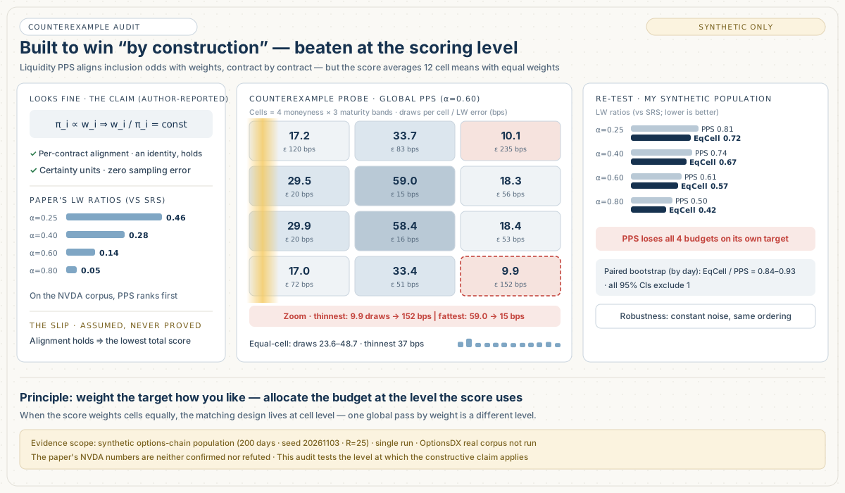
PPS does beat SRS (0.50–0.81; at α=0.80 its 95% interval vs SRS is [0.48, 0.52], equal-cell’s is [0.40, 0.44]), but it loses to equal-cell allocation at every α. In the paper, the same slot reads 0.46 / 0.28 / 0.14 / 0.05 — at α=0.80, PPS error is one twentieth of SRS. In my population, that dominance does not exist.

Precision first: this does not refute the paper’s NVDA numbers; magnitudes were never in claim scope. And two properties that get compressed into the single phrase “wins by construction” must be separated: when π is proportional to w, w/π is constant for non-certainty units and certainty units contribute no sampling error — that is an analytic identity, it holds in my population too, and I have not overturned it. What lost is the inference that slips out of the identity: the identity speaks of per-contract alignment, while the paper’s scoring (its Eq. 9) first computes the 12 cells’ LW means and then averages them with equal cross-cell weights, and the PPS budget is allocated once, globally, by weight — alignment at contract level, allocation at global level, scoring at cell level; when the three are not at the same level, the identity cannot underwrite the total score. My population’s contract density is in the paper corpus’s class (median 534 per day vs about 574), and the cross-cell total-weight gradient is steep (fattest-to-thinnest median 21.8×); the noise structure is admittedly coarser (my SRS RMSE starts at 288.5 bps vs the paper’s 124.0). One coupling also has to be excluded: my observation noise is generated proportional to spread, and the PPS weight has relative spread in its denominator, so high-weight contracts carry low noise by construction. I re-ran the whole set with spread-independent constant noise (mean-matched to the original): on the LW target, PPS posts 0.51–0.86 and equal-cell 0.35–0.52 — equal-cell is still lower at every budget. The coupling is excluded; what remains is the level mismatch itself.

The mechanism is visible at cell level. I audited my population’s structure: within-cell liquidity weight is concentrated — the top 5 contracts hold a median 0.56 share of cell weight — and at α=0.60 a median 165 contracts per day are PPS certainty units. In other words, the “PPS locks the weighted mean by grabbing the head contracts” route is open in my population too, and it still lost. Cells with small total weight also receive few draws, so their LW means rest on a handful of samples; equal-cell allocation floors every cell and tops up by dispersion, and coverage itself becomes precision. The per-cell decomposition supports this reading (α=0.60): under PPS the thinnest cell averages 9.9 draws with a cell LW error of 152 bps, the fattest 59 draws at 15 bps — a roughly 6× spread in draws across cells; equal-cell compresses draws into 23.6–48.7, with a thinnest-cell error of 37 bps. Nor is this “loss” a point-estimate mirage: pairing equal-cell and PPS day by day in a whole-day cluster bootstrap, the equal-cell/PPS ratios at the four α are 0.89 / 0.90 / 0.93 / 0.84, with 95% intervals [0.86, 0.92], [0.87, 0.94], [0.89, 0.97] and [0.80, 0.88] — none contains 1. I also self-checked the implementation first: on the LW target all four designs are scored with the same sample under the HT ratio estimator — sampling and scoring are two independent choices. The stratified designs post near-identical ratios on both targets (differences of 0.00–0.03) precisely because their allocations do not depend on the target: the same sample, rescored with a different normalising weight. Only PPS, whose inclusion probabilities are generated directly from w, flips with the target. In the NVDA corpus, global PPS’s within-cell precision happens to be high enough that the identity’s advantage cashes out as first place overall; that is the corpus’s distribution smoothing the level gap away, not a content of the identity itself. Put plainly: weight the target how you like — allocate the budget at the level the score uses. When scoring weights cells equally, the cell-level allocation is the design at the target’s level. This does not depend on any particular corpus; it is fixed by the protocol’s structure. Distributional conditions move the size of the gap, not the structural judgement.

This is also the paper’s most learnable methodological posture: the authors printed “by construction” in the open, which hands readers a falsifiable interface. My re-test simply used that interface.

The clock part: thinner tails, clustering intact

The paper’s second protocol is activity clocks: bars are cut not by fixed minutes but by volume or dollar volume, with thresholds causally calibrated on the trailing 60 trading days. Author-reported: under an 18.9× peak-to-trough price expansion, rolling volume/dollar clocks hold about 7.5–9.0 bars per day (interior-return basis 7.49 / 7.99, full-sample basis 8.49 / 8.99), interior excess kurtosis is pressed to 1.83 / 2.49 (time bars 5.00, diurnal-standardised 5.09); but lag-1 autocorrelation of squared returns stays at 0.170 / 0.215 — clustering unmoved; and next-bar direction accuracy is 48.6–51.0%, no alpha conjured from thin air either.

I re-tested on a synthetic intraday process over 320 trading days (U-shaped intraday seasonality, GARCH(1,1) minute variance, t5 shocks, jumps, 8.6× price expansion; the first 60 days calibrate, the rest are scored under the rolling 60-day protocol). One episode to disclose first: in the first version of the population, I set the volume coupling far too strong — extreme-volume days pushed the rolling thresholds so high that a typical day yielded only about 4 bars, and the process contained no intraday clustering to measure in the first place. That version was discarded before any verdict — on the basis of validity checks that precede any clock judgement (is the volume distribution sane, does clustering exist, is the bar rate in a scorable range); the changes touched only population parameters (a capped coupling, added GARCH), and the whole episode is on record. The revised results:

• Bar rate: rolling volume 9.40 ± 3.20 bars/day, segment means 10.1 / 9.1 / 9.7 — close to target (8.75 is the target frequency I pre-set for this synthetic population; the paper’s constant, calibrated on its own 967-session panel, is 8.273, and the 60-day rolling causal threshold mechanism is kept as-is); rolling dollar 11.28 ± 4.67, segments 12.3 / 10.8 / 11.6 with no time trend, but sitting about 30% above target (first reservation); in the control group, the static dollar threshold climbs over the same window from about 15 to about 53 (30.41 ± 18.29 overall) — rolling calibration stabilises the trend, not the level.
• Kurtosis: on the pooled aggregation the paper reports — rolling volume 0.69 (day-cluster bootstrap interval [0.15, 1.54]), rolling dollar 0.55 ([0.27, 0.81]), against time bars 8.73 and diurnal-standardised 6.83 ([3.02, 11.22]); both rolling clocks’ pooled kurtosis differences vs the diurnal control are −6.14 and −6.29 with intervals excluding 0, so the pooled compression holds; on the held-out last 40% of days both rolling clocks remain far below the controls (0.41 / 0.56 vs 12.64 / 8.18). But the per-day aggregation splits: volume’s per-day difference is −0.13 ([−0.22, −0.04]), supporting; dollar’s is +0.13 ([+0.02, +0.23]), reversed. So “thinner tails” holds for the volume clock under both aggregations, and for the dollar clock only under pooling (second reservation).
• Clustering and direction: pooled lag-1 autocorrelation of squared returns is positive under all six clocks (0.05–0.18); no clock presses it to zero. Next-bar direction accuracy is 0.493–0.510, overlapping the paper’s chance band. Be clear about what this item can show: my process has a conditional mean of zero by construction, so direction is unpredictable in principle; the check is not whether a clock can create predictability from nothing, but whether the clock transform manufactures spurious predictability — it does not.

The conclusion matches the authors’ own: activity clocks are a shaping tool for the unconditional distribution, not a cure for volatility dynamics, and not a signal source. Whoever reads a volume bar’s low kurtosis as “risk is gone” has mistaken reshaping for elimination.

What I did not test: the authors’ reported honesty

Two parts of the paper I did not touch, recorded here so readers know their grade (all author-reported):

In the longitudinal training-window sampling, PPS and Neyman at α=0.60 retain more tail-volatility windows (top-decile retention 81.2% / 73.7% vs SRS 59.9%), all three designs are equivalent to full training within a pre-set TOST margin, and 21–22% of compute time is saved; but the authors also report that the informative designs’ incremental forecasting gain over SRS is not established (paired tests p ≥ 0.608) — sampling saves compute, not accuracy.

The forecasting part is the classic case: HAR-IV posts a pooled MSE skill of +21.0%, the Tier-2 LSTM +17.2% while not beating HAR-IV (clustered DM test p=0.61). The authors themselves supply the concentration record: the top 5 trading days contribute 144–157% of the net squared-error improvement, the day-clustered test against the persistence benchmark is not significant (p=0.34), and persistence actually wins on 57.3% of days. Quoting the +21% on its own is a misreading of this paper — the authors printed the caveat on the same page as the number.

Four rules to take away

1. Write the target first, then choose the design. An equal-cell surface, a population mean and a liquidity-weighted surface are three different estimands, mapping to equal-cell, Neyman and PPS allocation respectively; the wrong design can double the error (mine 1.66–2.03×, the paper’s 2.47–3.90×).
2. Coverage is a hard metric (cell coverage). If the target is a per-cell quantity, any design that does not guarantee cell coverage must clear the coverage bar first; global probability sampling starving thin cells is the most common failure mode of a “constructive advantage”.
3. Align at the level the score uses. Constructive alignment is per-contract (π ∝ w is an identity); if scoring weights cells equally, the budget must be allocated at cell level — one global pass by weight is not at the same level as equal cross-cell scoring, and “unbeatable” has no foothold. Distributional conditions set the size of the gap, not this structural judgement.
4. Tail shaping is not elimination. Activity clocks press kurtosis and stabilise bar rates, but they do not move volatility clustering and produce no directional signal; when evaluating any “tail-taming” method, first ask whether it acts on the unconditional distribution or on conditional dynamics.

---

Evidence and replication note: the first-party numbers in this article come from two frozen-protocol runs on synthetic populations (options-chain population: 200 days, seed 20261103; intraday process: 320 days, seed 20261104), with the protocol re-implemented from the printed specifications in §3.1–3.2 and §5 of the paper; the chain arm’s parameters were frozen before any comparison, and the clock arm’s final specification was frozen after one pilot calibration (the v1 discard is on record) and not changed again before the final comparison. Full receipts, a claim-by-claim mapping and the code are public at github.com/vxime/iv-surface-sampling-replication (verifiable via SHA256SUMS). The OptionsDX real-corpus arm was not run — that corpus is obtained through the vendor store’s account and checkout flow, which was not authorised for this audit — so this article claims no real-corpus replication. The paper’s numbers (Bastola & Prushansky, arXiv:2610.33438v1) are all author-reported, and its longitudinal-equivalence and forecasting parts were not re-tested by me. This article discusses sampling and evaluation methodology only and is not investment advice.