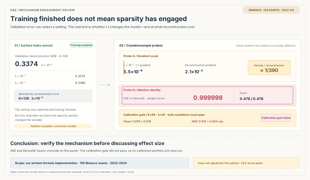
The first pair of models finished training, so I compared the SAE with its dense control (DenseAE, λ=0) by their weights. The weights are tied—the encoder and decoder share the same parameters—and their cosine similarity was 0.999998. In other words, the model with the sparsity penalty and the model without it were, for practical purposes, the same model. Hoyer sparsity (on a 0–1 scale, with larger values indicating greater sparsity) was 0.479 versus 0.478. Across the five folds, both had a prediction IC of +0.0073, and their portfolio results were almost indistinguishable.

I didn’t expect the first comparison to run into this. In the paper I was trying to reproduce, sparsity is the engine of the whole story: the L1 penalty is supposed to make the codes sparse, which in turn makes the portfolios selected by reconstruction rank less correlated and lowers their volatility. If sparsity never appears, numbers that look similar downstream are not actually validating the paper’s mechanism.

This article records the replication from end to end: what lined up, what did not, and—most importantly—where the evidence points when the results do not line up.

What the paper claims—and how strong each claim is

Han and Qu (University of Washington) had their paper accepted at ICAIF ‘26. The question is specific: feed daily cross-sectional returns into a single-layer sparse autoencoder, rank assets by its reconstruction values, form contrarian quintile portfolios, and ask whether risk falls because of sparsity itself.

The authors separate their main findings into three levels, and that distinction matters:

• Strictly confirmed: after selecting K=128 and λ=0.1 in advance on the first 748 days, the SAE portfolios had 20–26% lower rank-scale volatility than PCA with the same K across five confirmation folds.
• Exploratory: with K=64, volatility was 32–37% lower (20.0% versus 27.3% on the money-return scale). But the selection window overlapped with early test folds, so this is exploratory evidence only. The proposed mechanism was lower average pairwise correlation within the baskets: 0.008 versus 0.039 for PCA.
• Explicitly rejected by the authors: SAE added no Sharpe over the simplest same-day reversal baseline (a −2.48 gap on the money-return scale); factor identity did not reproduce across random seeds (decoder matching cosine 0.13 versus a random-dictionary reference of 0.117); and a Ledoit–Wolf minimum-variance overlay recovered about 73% of SAE’s volatility advantage over the naive baseline.

The authors also state three limitations themselves: signals are formed at the close on day t and executed at that same close, which they call “not practically executable”; costs are excluded throughout; and the crypto universe was filtered using full-sample information rather than point-in-time membership. There is another important omission: as of 2026-11-01, neither the paper nor its arXiv page linked to code, and the exact list of 433 assets was not published. Any replication therefore has to reimplement the printed protocol, and the panel is necessarily different. That determines what my conclusion can be: I am testing whether the claims transfer, not adjudicating whether the authors’ own run on their own panel was right or wrong.

My replication setup: deviations come first

I used daily Binance spot USDT klines from the public API. No account or API key was needed. The universe-freezing rule was fixed before training: 519 currently listed pairs, 285 with data in the 2022–2024 window, 245 with at least 252 observed days, then the top 150 by median daily quote volume. The list and its hash were saved before training. The number of eligible assets per day ranged from 89 to 150 (119 on average).

The deviations from the paper are explicit: 150 assets rather than 433, with my panel restricted to liquid assets; 2022–2024 rather than 2019–2024; and a universe drawn from pairs still trading today, which introduces survivorship tilt. The paper retained delisted assets through their last quote. Survivorship filtering systematically lowers volatility in this panel, and volatility is the central comparison in this article. The size of that bias cannot be reconstructed: delisted assets are no longer in the current trading list, so there is no way to count them from this source. Panel processing follows the paper: daily cross-sectional 1/99% winsorization, forward-fill missing values for at most three days and then mask them, and a clipped inverse-normal rank transform. The selection window uses the first 500 return days (450 training / 50 validation). Hyperparameters are selected only by validation reconstruction error over K∈{32,64,128} × λ∈{10⁻³,10⁻²,10⁻¹} × the learning-rate grid. After that come five expanding walk-forward folds, each with 119 signal days. The last signal day in each fold is excluded because its next-day return is needed for PnL, leaving 590 evaluation days. Portfolios are contrarian quintiles ranked by reconstruction, equal-weighted, with gross exposure of 1 per leg; missing t+1 returns are treated as zero. These choices match the paper.

I also preregistered two gates. The stop condition was simple: if the volatility direction did not reproduce on the reduced universe, report non-replication honestly; do not expand the universe or tune parameters until the sign changes. The calibration gate allowed one extra arm within the selection window if diagnostics showed that λ had failed to engage: choose a calibration λ using the criteria “sparsity target met and reconstruction cost controlled.” If no λ met both criteria, do not run the arm. The test set could not be used to change the rule after the fact.

The first problem: λ is inert on this panel

Start with hyperparameter selection. At K=128, validation reconstruction MSE is almost flat across λ: 0.3374 at λ=10⁻³, 0.3375 at 10⁻², and 0.3380 at 10⁻¹. The strict configuration selected by the rule is K=128, λ=10⁻³. On the authors’ panel, the same K was selected, but with the strongest λ=0.1. The same selection rule produced opposite preferences for penalty strength on the two panels. Selecting only by reconstruction error naturally favors the weakest penalty, because L1 can only make reconstruction harder; under that rule, my choice of 10⁻³ was almost inevitable. The paper, by contrast, reports selecting the strongest value, 0.1, under the same stated rule. That tension deserves to be recorded: either a strong penalty really did not hurt reconstruction on their panel, or some part of the selection process was not specified.

The gradient measurement is more direct. At λ=10⁻² (the paper’s exploratory setting), the mean magnitude of the L1 weight gradient is 5.5×10⁻⁶, compared with 2.1×10⁻³ for the reconstruction term. The penalty is only about 1/390 of the main gradient; they are not in the same range. In a separate diagnostic run—retrained on the first 500 days and evaluated on the first-fold window—I increased λ to 1.0, one hundred times the paper’s exploratory 10⁻², as a stress test. Hoyer moved only from 0.474 to 0.514. The model was still nowhere near sparse.

The calibration gate produced no qualifying λ. In a scan over λ∈{0.3,1,3,10,30} (this scan uses the K=64 selection-window setup), Hoyer rose from 0.483 to 0.619 and then saturated, while validation MSE climbed from 0.554 for the dense baseline to 0.918, a 66% increase. My gate required Hoyer to exceed DenseAE by at least 0.15 while keeping MSE within 1.2 times the dense baseline. At λ=30, Hoyer 0.619 just clears the 0.618 threshold (DenseAE’s 0.468 plus 0.15), but MSE 0.918 is about 1.4 times the allowed upper bound of 0.664. Under the preregistered rule, the calibration arm does not run. But “not enough penalty” explains only half the result: under the same protocol, the penalty gradient at λ=30 is already about 7.7 times the reconstruction gradient. The dose is more than strong enough, yet Hoyer still saturates around 0.62 and reconstruction breaks first. On this panel, λ values in the paper’s range are inert; beyond that range there is another ceiling. This architecture does not seem able to make the codes much sparser on this data while preserving reconstruction quality. The specific cause of that ceiling was not measured, so it remains uncertain.

Why can the same equation and the same λ grid reduce within-basket correlation to one-fifth on the paper’s panel, yet fail to change the model here? The measured part is clear: the relative scale of the penalty gradient and reconstruction gradient. Beyond that, I am making an inference and marking it as such. The relative strength of L1 depends on the typical scale of the code, and that scale changes with universe size and cross-sectional structure: the paper has 433 assets from 2019–2024; my panel has 150 liquid assets from 2022–2024. λ=0.1 may be an effective dose at their scale and effectively a placebo at mine. There is also an alternative explanation that cannot be ruled out: implementation details the authors have not released may make the actual penalty differ from the printed equation. One example is minibatch training; another is loss reduction. The printed equations do not specify whether the reconstruction term is summed or averaged over N assets, or whether the L1 term is summed or averaged over K hidden dimensions. The combination of those denominators alone could introduce hundreds-fold implicit scaling in the effective penalty. Without official code, this remains an open possibility; I cannot use it to reach a conclusion about the authors.

One thing does not depend on those inferences: under a standard implementation faithful to the printed equations, the paper’s λ values are not constants that can be carried from one panel to another without calibration. Anyone who copies λ=0.1 onto their own data and reports “the diversification effect of SAE” may be reporting a mechanism that never engaged.

Volatility keeps only its direction; the mechanism reverses

Five-fold aggregate results (590 days, money-return scale):

Method	Annualized volatility	Sharpe
Naive same-day reversal	31.39%	+1.69
PCA K=64	29.54%	+1.75
PCA K=128	30.39%	+1.32
SAE K=64 (λ=10⁻²)	29.90%	+0.65
SAE K=128 (λ=10⁻³, selected)	28.97%	+0.96
DenseAE K=64 (λ=0)	29.96%	+0.65

SAE-128 has 4.7% lower volatility than PCA-128 (fold by fold: −4.0, −4.2, +3.1, −3.0, −10.0; the direction matches in 4 of 5 folds). That is about one-fifth of the paper’s strict −20–26% result. The statistical detail matters too: the mean of the five fold-level differences is −3.6% (not the same quantity as the pooled −4.7%; one averages across folds, the other pools daily observations), with a t-statistic around −1.7 (n=5). It is not significant. The conclusion available here is limited to direction and magnitude. K=64 does not even preserve the direction: SAE volatility is 1.2% higher than PCA. Given the previous section, that is not surprising. The selected “SAE” at λ=10⁻³ is nearly dense, so its small advantage over PCA is more plausibly a property of ordinary autoencoder reconstruction than a benefit from sparsity.

To make the fold-level variation visible, these are the annualized money-volatility values in each fold:

Method	Fold 1	Fold 2	Fold 3	Fold 4	Fold 5
Naive reversal	22.12%	31.31%	32.00%	31.37%	37.93%
PCA K=64	21.71%	30.42%	27.16%	26.53%	39.22%
SAE K=64	20.16%	30.32%	30.54%	30.56%	35.91%
PCA K=128	21.65%	30.88%	29.05%	29.51%	38.26%
SAE K=128	20.78%	29.58%	29.95%	28.61%	34.42%

Mechanistically, the result is even clearer. Using the paper’s definition—average pairwise correlation within each basket on the rank scale with a trailing 60-day window—the SAE-64 long basket is 0.0215 and the short basket 0.0297; PCA-64 is 0.0201 / 0.0261; the naive reversal baskets are lower still at 0.0136 / 0.0148. The paper reports SAE 0.008 versus PCA 0.039. The ordering is reversed on my panel. On the raw-return scale, every method sits between 0.56 and 0.60 (the common market factor dominates), which also reveals no SAE advantage. Only one sub-finding points in the same direction as the paper: individual volatility of assets in the SAE baskets is slightly higher than in PCA (daily 0.0478 versus 0.0466). In other words, SAE did not simply pick quieter assets—but the assets it picked were not less correlated either.

My reading of the paper’s first claim is therefore: the direction appears partially at K=128, but the magnitude does not reproduce; K=64 and the mechanism claim do not reproduce. This does not falsify the authors’ result on their own panel—the panel, window, and implementation differ. It does show that the claim should not be treated as automatically portable across panels without calibration.

Some of the paper’s conclusions line up with my replication; others do not

One thing worth crediting in the paper is that the authors do not equate lower risk with tradable Alpha. They explicitly report no incremental Sharpe for SAE, factor identity that is unstable across random seeds, and no improvement in IC. They also disclose that same-close execution is not feasible, costs are excluded, and universe selection is not point-in-time. In my replication, the direction of those negative findings matches the authors’ report. But the sparsity separation does not reproduce, and the overlay cannot be judged cleanly because its construction is underspecified.

• No incremental Sharpe: the naive reversal has a money Sharpe of +1.69, versus +0.65 for SAE-64 and +0.96 for SAE-128. Prediction quality did not improve either: reversal IC is +0.0073 for SAE-64 versus +0.0146 for PCA-64 (the paper reports +0.016 versus +0.021, the same ordering).
• Factor identity does not reproduce across seeds: Hungarian matching across three seed pairs gives decoder cosine similarities of 0.217–0.220, against a random-dictionary reference of 0.198 (95th percentile 0.203). That is slightly above random—perhaps a shared market direction—but far from “the same set of factors.” The paper reports 0.13 versus 0.117. The magnitudes differ (the asset count differs, so the random baseline changes), but the conclusion is the same.
• Sparsity separation does not reproduce: the paper’s Hoyer values are 0.497 for SAE versus 0.303 for DenseAE; mine are 0.479 versus 0.478. Putting the pairs side by side shows where the gap comes from: the SAE side barely changes (0.497 versus 0.479); the entire missing separation is on the dense-baseline side (0.303 versus 0.478). I measured why: the exact-zero share of codes is 47.7% for SAE and 47.6% for DenseAE. On this panel, ReLU codes are already almost half zero without any penalty. The dense model is “sparse” by construction, so the gap disappears. This is another side of the previous finding: sparsity separation is present on the authors’ panel, but absent on mine.

I cannot give the overlay a clean verdict, so I will record it as it is. In the preregistered version—per-leg Ledoit–Wolf minimum-variance weights, raw-return covariance, money-return scale—volatility rose to 59.96% after the overlay because weights became too concentrated. In the rank-scale version, volatility was 8.19 (rank scale, not a percentage), below naive at 8.97 and below both SAE variants. The paper says only that a 60-day rolling LW covariance matrix is applied to the naive quintile portfolio; it does not pin down the construction. I cannot tell which of my two implementations, if either, is “theirs.” I broke down my own construction: each leg has about 28 assets, and the median condition number of the 60-day LW covariance matrix is about 94, so the matrix is not ill-conditioned. The problem is the weights: the minimum-variance solution concentrates each leg into about six effective holdings (median maximum single-name weight 27%). The 59.96% volatility is a consequence of concentrated weights, not a singular matrix. This remains inconclusive: the issue is on my replication side, and the construction details are not sufficiently specified.

With executable timing, returns disappear first; volatility does not move

The next section was not in the paper. It is my own extension, and its conclusions should not be attributed to the authors.

The paper’s evaluation forms a signal at the close on day t and executes at that same closing price. The authors themselves say this is not executable. I shifted the same baskets to the next day’s close (the earliest actually executable point in this setup) and added stylized costs of 10 / 25 bps based on turnover. Daily turnover is about 3.1 (the sum of absolute daily changes in combined long- and short-leg weights; the maximum is 4, so the portfolio is almost fully replaced every day):

Method	Same-close gross Sharpe	Next-close gross	Same-close net 10 bps	Next-close net 25 bps
SAE-128	+0.98	+0.05	−2.98	−10.07
SAE-64	+0.67	+0.26	−3.12	−9.34
Naive reversal	+1.71	−0.10	−1.86	−9.62

Note: Arm D was recomputed on 589 days using the stored baskets (one fewer day than the five-fold aggregate). That is why same-close Sharpe differs slightly from the aggregate table—for example, +0.98 versus +0.96 for SAE-128. The difference comes only from that one day.

Delaying execution by one day moves the gross Sharpe of all three methods close to zero. That is not surprising: daily reversal earns its money on the first day after the signal forms. Adding 10 bps of cost turns every result negative; at 25 bps, the losses are substantial. One qualification about market conventions: crypto trades 24/7 and has no closing auction. A “daily close” is just a snapshot at one point in time, so same-close execution with costs is actually the closer approximation to an executable setup (real latency and slippage would still need to be deducted). Next-close execution imports a conservative convention from equities. It measures an upper bound on the execution gap, not normal crypto-market behavior. Volatility barely changes across timing and cost variants, staying around 28–31%: costs are a smooth drag, while the timing shift removes the reversal premium itself. Neither changes the risk level.

The authors never claimed the strategy was tradable. This section quantifies the practical size of the disclaimer they did make: between “signal evidence” and a “tradable conclusion” sits an entire set of execution assumptions. Any daily cross-sectional model reporting Sharpe under same-close execution should pass this check before making stronger claims.

The checks I will run first when reviewing ML factor papers

This replication left me with a more durable checklist than the headline result. The order is now fixed:

1. Ablation identity check: turn off the claimed mechanism (λ=0 here) and compare weights, mechanism statistics (Hoyer here), and downstream metrics. If the two models are indistinguishable, report “mechanism did not engage” before discussing effect size. If I had run this check first, I could have avoided a long detour.
2. The simplest possible baseline: naive same-day reversal had the highest or nearly highest Sharpe on both panels. A complex model should beat it before we move on.
3. The textbook overlay: if a covariance overlay can recover most of the advantage, the model’s incremental contribution is only the residual. I could not reproduce this cleanly in this run, but the check still belongs in the protocol.
4. Seed stability: retrain with different seeds, match the factors, and compare against a random reference. If this fails, “we discovered factors” means only “this run produced some directions.”

Back to the 0.999998 from the opening. It is probably the most informative number in this replication. The paper’s equations, parameters, and evaluation protocol can all be copied word for word. Whether the mechanism actually engages is not written on the page; it has to be measured on your own panel. Whether volatility falls by a quarter or by 4.7%, until sparsity is confirmed, those are just numbers from a reconstruction model.

Replication boundary and materials: the conclusions here are limited to the reduced universe (150 liquid assets, 2022–2024, with survivorship tilt) and my own implementation of the printed equations (NumPy, with finite-difference gradient checks). This article neither confirms nor refutes the authors’ results on their 433-asset 2019–2024 panel. The data are public Binance daily klines and can be rebuilt using the rules described above. The authors’ official code had not been published at the time of writing. Paper figures cited here are labeled as author-reported. This article discusses replication methods and evidence boundaries only; it is not investment advice.

The replication code, frozen asset list (with hashes), fold-level results, and interpretation notes are public. The materials include SHA256SUMS so each file can be checked individually.

vxime/sae-crypto-factor-replication

If you want to place this replication in a broader quantitative research workflow, see How to validate whether a quantitative factor is useful and How to adjust multi-factor model weights safely. The first asks whether ranking evidence holds; the second looks at how to control model-weight changes once that evidence enters a system.