# 114 Executions at One Nanosecond: Where Hawkes Likelihood Goes Wrong

> Canonical: https://vxi.me/en/posts/hawkes-itch-nanosecond-ties-likelihood/
> Locale: en-us
> Published: 2026-10-31
> Updated: 2026-10-31
> Markdown: https://vxi.me/en/posts/hawkes-itch-nanosecond-ties-likelihood.md

<figure class="hawkes-ties-hero not-prose" lang="en-us">
<picture>
  <source media="(prefers-reduced-motion: reduce) and (max-width: 640px)" srcset="/images/posts/hawkes-itch-nanosecond-ties-likelihood/hawkes-tie-scores.mobile.still.en-us.svg" type="image/svg+xml">
  <source media="(prefers-reduced-motion: reduce)" srcset="/images/posts/hawkes-itch-nanosecond-ties-likelihood/hawkes-tie-scores.still.en-us.svg" type="image/svg+xml">
  <source media="(max-width: 640px)" srcset="/images/posts/hawkes-itch-nanosecond-ties-likelihood/hawkes-tie-scores.mobile.en-us.svg" type="image/svg+xml">
  <img src="/images/posts/hawkes-itch-nanosecond-ties-likelihood/hawkes-tie-scores.en-us.svg" alt="Hawkes toy scoring of 114 equal-timestamp events: pre-batch event term 183.475922 nats; row-ordered 396.770155 nats, 213.294233 nats higher. Both share a 48.237046-nat compensator." width="1200" height="700" loading="eager" fetchpriority="high" decoding="async" style="display:block;width:100%;height:auto">
</picture>
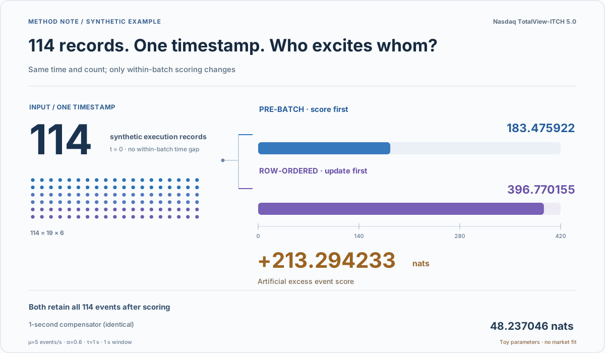
<figcaption>Figure: two scoring rules for one synthetic batch; not an AAPL market-parameter fit.</figcaption>
</figure>

One number in a Nasdaq ITCH sample made me stop before handing the stream to a conventional event-by-event Hawkes loop: **114**.

In the July 30, 2019 AAPL regular-session data, one nanosecond timestamp contains 114 `execution` message rows; batches of 131 and 187 also occur once each. Of **49,172 execution-class messages, 30,080 (61.17%) share a timestamp** with another record. Ties are common; batches in the hundreds are not. These rows are events *under our study's definition*, not 114 distinct orders or proof that physical executions happened simultaneously.

The trap is straightforward. If code updates Hawkes excitation after each input row, row 114 receives excitation from the preceding 113 rows even though all recorded time differences are zero. With asymmetric cross-type excitation, even the order of types within the file can change the score. **Which within-batch temporal assumption should a model be allowed to make?**

We fixed the rule *before* fitting: batch by **symbol + integer nanosecond timestamp**, score every member using the state just before the batch, and only then update the state with the actual counts. The exchange's transmitted message order is real information; treating it as sub-nanosecond physical time, without an explicit observation model, is not.

That yields three useful code-review questions: Is the grouping key correct? Is history updated only after batch scoring, without discarding multiplicity? Does the compensator cover the complete observation session?

## Timestamp ties are common; 114 is an extreme tail batch

The [official Nasdaq TotalView-ITCH 5.0 specification](https://nasdaqtrader.com/content/technicalsupport/specifications/dataproducts/NQTVITCHSpecification.pdf) describes the timestamp as nanoseconds since midnight. Message `E` means Order Executed and `C` means Order Executed With Price; a single order reference can also be involved in multiple partial execution messages.

Our three modeling classes are **`add=A/F`**, **`cancel_delete=X/D`** and **`execution=E/C`**, grouped by symbol, type and integer-nanosecond timestamp. The `C` class includes both `Printable=Y` and `Printable=N`; this is **not** a count of printable trades alone. `P` (trade involving a non-displayed order) and `Q` (cross trade) are excluded. That mapping is the researcher's definition, not Nasdaq's universal taxonomy of all transactions.

The following internally inspected aggregate covers **AAPL on 2019-07-30, 09:30–16:00 US Eastern exchange time** (the full regular session):

| Metric | Observed value |
| --- | ---: |
| `execution` message records | 49,172 |
| Distinct nanosecond timestamps | 29,379 |
| Timestamps with multiple records | 10,287 |
| Records on tied timestamps | 30,080 (61.17%) |
| Median / mode of tied-batch size | 2 / 2 records |
| Tied batches of size 2–3 | 8,439 (82.04% of tied batches) |
| Timestamps with exactly 114 records | 1 |
| Larger batches of 131 / 187 records | 1 each |


Do not confuse this session with an earlier **09:30–11:00** common-window comparison. The saved aggregate tells us batch sizes, not the individual order identities or their unobservable physical ordering.

Across all 29,379 timestamps, the mean is **1.67 records per timestamp**. Among the 10,287 tied batches, the mean is **2.92**, and both the median and mode are **2**. A batch of 114 is around **39 times** that latter mean. Only three tied batches reach at least 114 records (114, 131 and 187). The tail exposes a numerical trap but is not a typical batch.

The high tied-row share also means this pre-batch convention does not use unobserved within-batch gaps to identify self- or cross-excitation. Identifiability still depends on intervals between batches and type composition; **61.17% alone does not prove that parameters are unidentifiable**.

## At the same timestamp, which event may excite which?

For three event types with an exponential Hawkes kernel, write the conditional intensity as:

```text
lambda_k(t-) = mu_k(t)
             + sum_j [alpha[k,j] / tau
               * sum_{u<t} m_j(u) * exp(-(t-u)/tau)]
```

Here `k` denotes the target and `j` the source. `m_j(u)` is the true number of source-type rows recorded at timestamp `u`; matrix orientation is **target × source**. `mu_k` has units events/s, `tau` is measured in seconds, and `alpha[k,j]` is the dimensionless integrated excitation per source event. Consequently the instantaneous kernel coefficient is `alpha[k,j]/tau`, while its time integral contains `alpha`.

The crucial restriction is **`u<t`**. Under our pre-batch convention, events stamped `t` cannot enter the history used to score their own batch. Its event contribution becomes:

```text
event_term(t) = sum_k m_k(t) * log(lambda_k(t-))
```

Compute every `lambda_k(t-)` from the same prior state, sum log intensity weighted by the full event counts, then update history once with `m_add`, `m_cancel_delete` and `m_execution`. A batch of 114 is not one event. Useful synthetic regression cases permute row order, isolate symbols and reset history across sessions.

Sequential scoring in transmitted-message order *could* be a separate modeling decision, but only if its time/observation assumptions are stated. It must not be presented as a faster implementation of the same likelihood.

## A 114-row toy example exposes the difference

This is **not a fitted AAPL model**. It is an executable Python-standard-library illustration: 114 same-type events at session start, no prior excitation, `mu=5` events/s, `alpha=0.6`, `tau=1` s, followed by one second of observation.

```python
import math

m, mu, alpha, tau, horizon = 114, 5.0, 0.6, 1.0, 1.0

# Score every event at the pre-batch intensity
pre_batch = m * math.log(mu)

# Counterexample: let prior rows at the same timestamp excite later rows
row_ordered = math.fsum(
    math.log(mu + alpha * i / tau) for i in range(m)
)

# Full likelihood subtracts integrated intensity over the entire window
baseline_area = mu * horizon
excitation_area = alpha * m * (-math.expm1(-horizon / tau))
compensator = baseline_area + excitation_area

print(f"prebatch_event_log_term: {pre_batch:.6f}")
print(f"row_ordered_event_log_term: {row_ordered:.6f}")
print(f"artificial_excess: {row_ordered - pre_batch:.6f}")
print(f"one_second_compensator: {compensator:.6f}")
print(f"one_second_full_LL: {pre_batch - compensator:.6f}")
```

Run in an isolated Linux environment with Python 3.13.5 (exit code 0), it produced:

```text
prebatch_event_log_term: 183.475922
row_ordered_event_log_term: 396.770155
artificial_excess: 213.294233
one_second_compensator: 48.237046
one_second_full_LL: 135.238876
```

Merely allowing earlier rows in the *same recorded instant* to excite later ones increases the event log term by **213.294233 nats**. Both approaches nevertheless retain **the same 114 events in post-batch history**. Since this example's batch has zero duration, the subsequent one-second compensator is identical: **48.237046 nats**. The row-ordered full score is **348.533109**, versus **135.238876** for pre-batch—a difference of **213.294233 nats**.

This is a numerical comparison of two **working scoring conventions**, not a realized improvement in prediction and not two exact likelihoods for a common continuous-time observation model. Nor does pre-batch discard future excitation: one second later those 114 events contribute `114 × 0.6 × exp(-1) ≈ 25.163` events/s under the toy assumptions.

## Event terms alone are not the full likelihood

Summing `log(lambda)` over arrivals is only half the accounting. A point-process log likelihood also subtracts the integrated intensity over the *entire* valid observation window:

```text
LL = sum_k sum_batches m_k(t) * log(lambda_k(t-))
     - sum_k integral_session lambda_k(t) dt
```

Before fitting, our study fixed an intraday baseline of **78 five-minute intervals** across the 390 minutes from 09:30 to 16:00. A baseline segment contributes exactly its half-open overlap with the session; every past batch contributes its actual multiplicity to the integrated exponential kernel:

```text
baseline_area[k] = sum_r mu[k,r] * overlap_seconds(r, session)

excitation_area[k] = sum_j sum_{u in session}
    alpha[k,j] * m_j(u) * (1 - exp(-(end-u)/tau))
```

The code uses `-expm1(-(end-u)/tau)` to avoid cancellation for short intervals. In the one-second toy case, baseline area is `5`, integrated excitation about `43.237046`, and total compensator **48.237046**. Thus full pre-batch LL is **135.238876**, not merely the event term **183.475922**. Without the compensator, there is no penalty for maintaining intensity through the observation interval.

## What can the real batch histogram say about scenario sensitivity?

The toy shows *how* row-order self-excitation inflates a score. We then used an **already stored 2019-07-30 full-session AAPL execution batch-size histogram** as multiplicity input to *artificial-parameter* scenarios. No raw ITCH messages were re-downloaded or refitted.

Assume only **positive self-excitation of the execution class**, and suppose its intensity just before each batch, `lambda^-`, is at least an artificially specified `mu>0`. For a batch with `m` rows, the increment from row-wise within-timestamp self-excitation satisfies:

```text
0 <= Delta(m) = sum_{i=0}^{m-1} log(1 + alpha*i/(tau*lambda^-))
   <= sum_{i=0}^{m-1} log(1 + alpha*i/(tau*mu))
```

The right-hand expression is a **conditional upper bound for the same-type scenario**, *not* a bound on a fitted full three-type Hawkes LL. Actual pre-batch intensities and other simultaneous event types are not present in this calculation.

At `mu=5` events/s, the aggregate conditional bounds over the saved multiplicity histogram are:

| Artificial alpha | tau=0.1 s | tau=1 s | tau=10 s |
| --- | ---: | ---: | ---: |
| 0.1 | 8,392.65 | 1,436.32 | 178.46 |
| 0.3 | 17,088.26 | 3,472.79 | 500.41 |
| 0.6 | 25,186.19 | 5,837.61 | 928.45 |


All entries are in **nats**, and the parameters are hypothetical. At `mu=5, alpha=0.3, tau=1`, the cumulative upper bound is **3,472.79 nats**, or **0.0706 nats per record when divided by the 49,172 execution records**. Under that assumption a typical two-row tied batch contributes an upper bound of **0.0583 nats**; a three-row batch, **0.1716 nats**. Changing the assumed lower bound `mu` to 1 or 20 produces **11,044.42** or **1,125.70 nats**.

Across the nine displayed parameter combinations, the conditional bounds run from **178.46 to 25,186.19 nats** (about **0.00363–0.51221 nats/record**). They cannot tell us the actual AAPL likelihood error, let alone a market-fitted Hawkes parameter.

Removing the largest batches shows how much the extreme tail contributes *within this one artificial scenario*:

| Largest batches excluded | Upper-bound decrease (nats) | Share of original bound |
| --- | ---: | ---: |
| 187 records (top 1) | 321.54 | 9.26% |
| 187, 131, 114 (top 3) | 665.62 | 19.17% |
| Largest 10 batches | 1,123.57 | 32.35% |


The three largest batches contain only **432 rows** but supply about a fifth of this conditional upper bound. The stored histogram has **no timestamps for those extreme batches**, so we cannot attribute them to market open, close, matching mechanics or timestamp encoding.

The histogram counts were reconciled with the original stored aggregate. A distinct **13/13** synthetic-and-aggregate test slice covers the 114-row arithmetic, monotonicity, top-k identity and directory-layout reproduction; the earlier **99** synthetic research checks were run separately.

## What actually passed in testing?

The real AAPL aggregate establishes the *existence and size* of timestamp ties. Known-parameter synthetic experiments test whether batch scoring, state updates and compensators follow their mathematical contract. Neither should be mistaken for market model fitting.

| Synthetic test group | What was checked |
| --- | --- |
| Batch scoring (10) | Shared pre-batch intensity; multiplicities retained; row permutation invariance |
| Full likelihood (33) | Baseline and kernel compensators; analytic vs numerical integration |
| M0/M1/M2 contracts (34) | Homogeneous Poisson, 78-bin seasonal NHPP and three-type Hawkes under known parameters |
| Synthetic event streams (22) | Seeded Ogata thinning; independent history sums; two-process determinism |
| Total | **99/99 research-slice tests passed** (Python 3.13.5, isolated Linux x86_64) |


One deterministic stress fixture contains **209 synthetic events in four timestamp groups**: 90 Adds at session start; 114 Executions at +1 s; 3 Cancel/Delete at +2 s; then 1 Add and 1 Execution together at +3 s. The group counts are **90/114/3/2**. Against independently written direct history-summation/integration code, the maximum absolute discrepancy was about `1.42e-14`; reversing input order did not change the result.

Two separately simulated Ogata-thinning continuous-time streams contained **285 and 265** events. Their independent likelihood comparison differed by at most about `7.11e-15`. Those simulations did **not naturally produce 114 exact timestamp ties**; the 114-row fixture was deliberately constructed.

The research tests ran on isolated Linux x86_64 with Python 3.13.5, with historical receipts. **They do not constitute a successful Actions run on the current editorial HEAD.** No real-market model fitting, held-out scoring or claim of Hawkes outperforming seasonal NHPP has been established.

## Why this is a working likelihood, not a proven exact density

A simple continuous-time point process normally has zero probability of exact ties. ITCH nanosecond marks are recorded/encoded timestamps, not a direct view of finer physical arrival times. The **pre-batch working likelihood (or pseudo-likelihood score)** is therefore a stated observational convention, not a derived exact joint density for rounded timestamps. Calling it a `composite likelihood` without specifying component densities and dependence is also unjustified.

For fixed-time-bin counts one might build a discrete-time count model; to infer unobserved within-bin arrivals one needs interval-censoring assumptions. Ordering small ties can be a sensitivity analysis, not a one-line universal substitute.

One algebraic point matters for model comparisons. If two scores under **the same data, grouping and observation-model definition** omit an identical parameter-independent constant `C(D)`, that constant cancels from their *difference*: `(LL_A+C(D))-(LL_B+C(D))=LL_A-LL_B`. An example under certain discrete count models is a `-sum log(m!)` term. Cancellation does not preserve absolute LL and adding a factorial term alone does not turn pre-batch scores into an exact observation likelihood. Change the grouping or time convention and the constant need not match.

Even under one scoring convention, a standard chi-square likelihood-ratio test is not automatically valid: nonnegative excitation parameters sit at a boundary, and decay parameters may be unidentifiable under the null.

## How to inspect residuals when timestamps tie

Treating 114 rows at one timestamp as 114 ordered arrivals gives a pile of zero interarrival durations and distorts time-rescaling diagnostics. The pre-registered plan instead groups **unique timestamps per event type** for residual analyses, while reporting each batch multiplicity separately. QQ plots, residual autocorrelation and KS distances describe mismatch; ordinary continuous-arrival KS `p`-values are **not formal inference here**. Any future bootstrap/permutation procedure must first define its null, generator and dependence-preserving resampling unit.

That check comes before selecting an impressive Hawkes estimate. **Input-file row order must not quietly become causal event time.**

Public reproduction materials: [Python scripts, histogram, tests and SHA-256 checks](/evidence/hawkes-itch-nanosecond-ties-likelihood/README.md).

## Verification context

- Level: first-party
- Verified: 2026-10-31T00:00:00.000Z
- Environment: Python 3.13.5; Linux x86_64; historical synthetic research tests
- Environment: Python 3 standard-library public reproducer and aggregated histogram
- Evidence mode: mixed
- Evidence receipt: https://vxi.me/evidence/hawkes-itch-nanosecond-ties-likelihood.json